Audio Data Augmentations¶

In this chapter, we will discuss common transformations that we can apply to audio signals in the time domain. We will refer to these as “audio data augmentations”.

Data augmentations are a set of methods that add modified copies to a dataset, from the existing data. This process creates many variations of natural data, and can act as a regulariser to reduce the problem of overfitting. It can also help deep neural networks become robust to complex variations of natural data, which improves their generalisation performance.

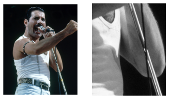
In the field of computer vision, the transformations that we apply to images are often very self-explanatory. Take this image, for example. It becomes clear that we are zooming in and removing the color of the image:

import numpy as np
from PIL import Image

with Image.open("../../book/images/janne/freddie_mercury.jpg") as img:
    img = np.array(img)
    fig, ax = plt.subplots(1, 2)
    ax[0].imshow(img)
    h, w, c = img.shape
    cropped_img = img[int(h / 2) : int(h / 2) + 500, int(w / 2) : int(w / 2) + 400, :]
    black_white_img = cropped_img[..., 0]
    ax[1].imshow(black_white_img, cmap="gray")
    ax[0].axis("off")
    ax[1].axis("off")
    plt.show()

Naturally, we cannot translate transformations from the vision domain directly to the audio domain. Before we explore a battery of audio data augmentations, we now list the currently available code libraries:

Code Libraries¶

Name	Author	Framework	Language	License	Link
Muda	B. McFee et al. (2015)	General Purpose	Python	ISC License	source code
Audio Degradation Toolbox	M. Mauch et al. (2013)	General Purpose	MATLAB	GNU General Public License 2.0	source code
rubberband	-	General Purpose	C++	GNU General Public License (non-commercial)	website, pyrubberband
audiomentations	I. Jordal (2021)	General Purpose	Python	MIT License	source code
tensorflow-io	tensorflow.org	TensorFlow	Python	Apache 2.0 License	tutorial
torchaudio	pytorch.org	PyTorch	Python	BSD 2-Clause “Simplified” License	source code
torch-audiomentations	Asteroid (2021)	PyTorch	Python	MIT License	source code
torchaudio-augmentations	J. Spijkervet (2021)	PyTorch	Python	MIT License	source code

Listening¶

One of the most essential, and yet overlooked, parts of music research is exploring and observing the data. This also applies to data augmentation research: one has to develop a general understanding of the effect of transformations that can be applied to audio. Even more so, when transformations are applied sequentially.

For instance, we will understand why a reverb applied before a frequency filter will sound different than when the reverb is applied after the frequency filter. Before we develop this intuition, let’s listen to a series of audio data augmenations.

import os
import random

import numpy as np
import soundfile as sf
import torch
from torch.utils import data
from torchaudio_augmentations import (
    Compose,
    Delay,
    Gain,
    HighLowPass,
    Noise,
    PitchShift,
    PolarityInversion,
    RandomApply,
    RandomResizedCrop,
    Reverb,
)

GTZAN_GENRES = [
    "blues",
    "classical",
    "country",
    "disco",
    "hiphop",
    "jazz",
    "metal",
    "pop",
    "reggae",
    "rock",
]


class GTZANDataset(data.Dataset):
    def __init__(self, data_path, split, num_samples, num_chunks, is_augmentation):
        self.data_path = data_path if data_path else ""
        self.sr = 22050
        self.split = split
        self.num_samples = num_samples
        self.num_chunks = num_chunks
        self.is_augmentation = is_augmentation
        self.genres = GTZAN_GENRES
        self._get_song_list()
        if is_augmentation:
            self._get_augmentations()

    def _get_song_list(self):
        list_filename = os.path.join(self.data_path, "%s_filtered.txt" % self.split)
        with open(list_filename) as f:
            lines = f.readlines()
        self.song_list = [line.strip() for line in lines]

    def _get_augmentations(self):
        transforms = [
            RandomResizedCrop(n_samples=self.num_samples),
            RandomApply([PolarityInversion()], p=0.8),
            RandomApply([Noise(min_snr=0.3, max_snr=0.5)], p=0.3),
            RandomApply([Gain()], p=0.2),
            RandomApply([HighLowPass(sample_rate=22050)], p=0.8),
            RandomApply([Delay(sample_rate=22050)], p=0.5),
            RandomApply(
                [PitchShift(n_samples=self.num_samples, sample_rate=22050)], p=0.4
            ),
            RandomApply([Reverb(sample_rate=22050)], p=0.3),
        ]
        self.augmentation = Compose(transforms=transforms)

    def _adjust_audio_length(self, wav):
        if self.split == "train":
            random_index = random.randint(0, len(wav) - self.num_samples - 1)
            wav = wav[random_index : random_index + self.num_samples]
        else:
            hop = (len(wav) - self.num_samples) // self.num_chunks
            wav = np.array(
                [
                    wav[i * hop : i * hop + self.num_samples]
                    for i in range(self.num_chunks)
                ]
            )
        return wav

    def __getitem__(self, index):
        line = self.song_list[index]

        # get genre
        genre_name = line.split("/")[0]
        genre_index = self.genres.index(genre_name)

        # get audio
        audio_filename = os.path.join(self.data_path, "genres", line)
        wav, fs = sf.read(audio_filename)

        # adjust audio length
        wav = self._adjust_audio_length(wav).astype("float32")

        # data augmentation
        if self.is_augmentation:
            wav = (
                self.augmentation(torch.from_numpy(wav).unsqueeze(0)).squeeze(0).numpy()
            )

        wav = torch.from_numpy(wav.reshape(1, -1))
        return wav, self.sr, genre_index

    def __len__(self):
        return len(self.song_list)


def get_dataloader(
    data_path=None,
    split="train",
    num_samples=22050 * 29,
    num_chunks=1,
    batch_size=16,
    num_workers=0,
    is_augmentation=False,
):
    is_shuffle = True if (split == "train") else False
    batch_size = batch_size if (split == "train") else (batch_size // num_chunks)
    data_loader = data.DataLoader(
        dataset=GTZANDataset(
            data_path, split, num_samples, num_chunks, is_augmentation
        ),
        batch_size=batch_size,
        shuffle=is_shuffle,
        drop_last=False,
        num_workers=num_workers,
    )
    return data_loader

from torchaudio.datasets import GTZAN

train_loader = get_dataloader(
    data_path="../../codes/split", split="train", is_augmentation=False
)
dataset = train_loader.dataset
idx = 5
print(f"Number of datapoints in the GTZAN dataset: f{len(dataset)}\n")
print(f"Selected track no.: {idx}")
audio, sr, genre = dataset[idx]
print(
    f"Genre: {genre}\nSample rate: {sr}\nChannels: {audio.shape[0]}\nSamples: {audio.shape[1]}"
)
display(Audio(audio, rate=sr))

Number of datapoints in the GTZAN dataset: f442

Selected track no.: 5
Genre: 0
Sample rate: 22050
Channels: 1
Samples: 639450

Random Crop¶

Similar to how we can crop an image, so that only a subset of the image is represented, we can ‘crop’ a piece of audio by selecting a fragment between two time points $t_0 - t_1$.

Various terms for this exist, e.g.,: slicing, trimming,

Frequency Filter¶

Note

In these examples and the accompanying code, we assume the shape of audio ordered in our array is follows: (channel, time)

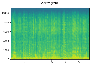
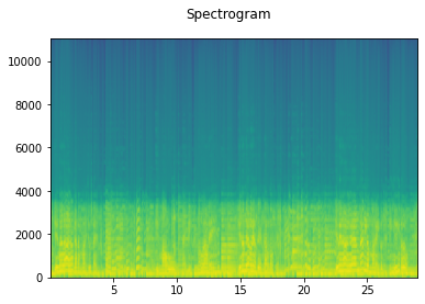
A frequency filter is applied to the signal. We can process the signal with either the LowPass or HighPass algorithm [47]. In a stochastic setting, we can determine which one to apply by, for example, a coin flip. Another filter parameter we can control stochastically is the cutoff frequency: the frequency at which the filter will be applied. All frequencies above the cut-off frequency are filtered from the signal for a low-pass filter (i.e., we let the low frequencies pass). Similarly for the high-pass filter, all frequencies below the cut-off frequency are filtered from the signal (i.e., we let the high frequencies pass).

from torch_audiomentations import LowPassFilter

taudio = LowPassFilter(
    sample_rate=sr,
    p=1.0,
    min_cutoff_freq=3000,
    max_cutoff_freq=3001,
)(audio.unsqueeze(0)).squeeze(0)

print("Original")
display(Audio(audio, rate=sr))
plot_spectrogram(audio, sr)

print("LowPassFilter")
display(Audio(taudio, rate=sr))
plot_spectrogram(taudio, sr)

Original

LowPassFilter

Delay¶

The signal is delayed by a value that can be chosen arbitrarily. The delayed signal is added to the original signal with a volume factor, e.g.,, we can multiply the signal’s amplitude by 0.5.

from torchaudio_augmentations import Delay

taudio = Delay(sample_rate=sr, min_delay=200, max_delay=201)(audio)
print("Original")
display(Audio(audio, rate=sr))
# plot_spectrogram(audio, sr)

print(f"Delay of {200}ms")
display(Audio(taudio, rate=sr))
# plot_spectrogram(taudio, sr)

Original

Delay of 200ms

Comb filter¶

When we apply a delayed signal to the original with a short timespan and a high volume factor, it will cause interferences. These audible interferences are called a “comb filter”.

from torchaudio_augmentations import Delay

taudio = Delay(sample_rate=sr, min_delay=60, max_delay=61)(audio)
print("Original")
display(Audio(audio, rate=sr))
# plot_spectrogram(audio, sr)

print(f"Delay of {61}ms")
display(Audio(taudio, rate=sr))
# plot_spectrogram(taudio, sr)

Original

Delay of 61ms

Pitch Shift¶

The pitch of the signal is shifted up or down, depending on the pitch interval that is chosen beforehand. Here, we assume a 12-tone equal temperament tuning that divides a single octave in 12 semitones.

from torchaudio_augmentations import PitchShift

taudio = PitchShift(
    sample_rate=sr, n_samples=audio.shape[1], pitch_cents_min=4, pitch_cents_max=5
)(audio)
print("Original")
display(Audio(audio, rate=sr))
# plot_spectrogram(audio, sr, title="Original")

print(f"Pitch shift of {4} semitones")
display(Audio(taudio, rate=sr))
# plot_spectrogram(taudio, sr, title="Pitch shift")

Original

Pitch shift of 4 semitones

Reverb¶

To alter the original signal’s acoustics, we can apply a Schroeder reverberation effect. This gives the illusion that the sound is played in a larger space, in which it takes longer for the sound to reflect.

Applying a reverberation of a “small” room on a signal that was recorded in a larger room does not have the opposite effect: the process of reverberation is an additive process. The reverse process is called “dereverberation”.

from torchaudio_augmentations import Reverb

taudio = Reverb(
    sample_rate=sr,
    reverberance_min=90,
    reverberance_max=91,
    room_size_min=90,
    room_size_max=91,
)(audio)
print("Original")
display(Audio(audio, rate=sr))
# plot_spectrogram(audio, sr, title="Original")

print(f"Reverb")
display(Audio(taudio, rate=sr))
# plot_spectrogram(taudio, sr, title="Reverb")

Original

Reverb

Gain¶

Warning

In Jupyter notebook’s Audio() object, we have to set normalize=False so that we can hear an unnormalized version of the audio. This is important to reflect the true audio transformation output.

We can apply a volume factor to the signal, so that it is perceived as louder. It is generally accepted that a loudness gain of 10 decibels is perceived as twice as loud, and similarly 10 decibels of gain reduction is perceived half as loud.

from torchaudio_augmentations import Gain

taudio = Gain(min_gain=-16, max_gain=-15)(audio)
print("Original")
display(Audio(audio, rate=sr))
# plot_spectrogram(audio, sr, title="Original")

print(f"Gain")
display(Audio(taudio, rate=sr, normalize=False))
# plot_spectrogram(taudio, sr, title="Gain")

Original

Gain

Noise¶

White Gaussian noise is added to the complete signal with a signal-to-noise ratio (SNR) that can be specified. A uniform distribution between the minimum and maximum SNR boundaries is made so that, for example, we can draw a different SNR value for each example in a mini-batch during training.

from torchaudio_augmentations import Noise

taudio = Noise(min_snr=0.04, max_snr=0.04)(audio)
print("Original")
display(Audio(audio, rate=sr))
# plot_spectrogram(audio, sr, title="Original")

print(f"Noise")
display(Audio(taudio, rate=sr, normalize=True))
# plot_spectrogram(taudio, sr, title="Noise")

Original

Noise

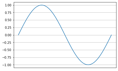
Polarity Inversion¶

While this does not have an effect on a time-frequency representation of audio, e.g., a spectrogram, encoders that are trained on raw waveforms can benefit from an audio data augmentation that flips the phase of an audio signal: Polarity Inversion. Simply put, the signal is multipled by $-1$, which causes the phase to invert.

Interestingly, when we add the original signal to the phase-inverted signal, all phases will cancel out. This will naturally result in silence. This is the core principle behind noise-cancelling headphones, which record the sound of your surroundings and apply a polarity inversion as to reduce unwanted noise.

import math

l = 1 / 440.0
test_audio = torch.sin(math.tau * 440.0 * torch.linspace(0, l, int(l * sr))).unsqueeze(
    0
)
plt.plot(test_audio.squeeze(0))
plt.grid()
plt.xticks([])
plt.show()

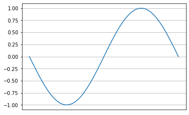
inverted_test_audio = PolarityInversion()(test_audio)
plt.plot(inverted_test_audio.squeeze(0))
plt.grid()
plt.xticks([])
plt.show()

from torchaudio_augmentations import PolarityInversion

taudio = PolarityInversion()(audio)
print("Original")
display(Audio(audio, rate=sr))
# plot_spectrogram(audio, sr, title="Original")

print(f"Polarity Inversion")
display(Audio(taudio, rate=sr, normalize=True))
# plot_spectrogram(taudio, sr, title="Polarity Inversion")

print(f"Original + Polarity Inversion")
display(Audio(audio + taudio, rate=sr, normalize=True))
# plot_spectrogram(audio + taudio, sr, title="Original + Polarity Inversion")

Original

Polarity Inversion

Original + Polarity Inversion

Sequential Audio Data Augmentations¶

Now that we have built up some intuition of some of the audio transformations, let us observe how they can be applied sequentially. More importantly, to develop an understanding on how different audio transformations interact when we apply them before, or after each other.

For this, we can use a Compose module, which takes as input a list of audio transformations. These will be applied in the order they appear in the supplied list. This interface is similar to torchvision.transforms and torchaudio.transforms’ Compose modules.

from torchaudio_augmentations import Compose, HighLowPass

transform = Compose([Delay(sample_rate=sr), HighLowPass(sample_rate=sr)])
transformed_audio = transform(audio)
print("Original:")
display(Audio(audio, rate=sr))
print("Transform:", transform)
display(Audio(transformed_audio, rate=sr))

Original:

Transform: Compose(
	Delay()
	HighLowPass()
)

Now that we have listened to what a sequential audio transformation sounds like, let’s observe how two different transforms interact when they are applied in a different sequential order.

Let’s take the following two transforms:

Noise
Reverb

A signal that does not have any reverberation added, is commonly called a dry signal. A signal that is reverberated is called a wet signal.

When we first apply the Noise transform, the Reverb transform will apply the reverberation to the dry signal and the added noise signal. This will result in a completely wet signal.

Conversely, when we first apply the Reverb transform, the Noise signal will be added after the reverberated signal. The noise is thus dry, i.e., it is not reverberated.

from torchaudio_augmentations import Compose

noise = Noise(min_snr=0.05, max_snr=0.06)
reverb = Reverb(
    sample_rate=sr,
    reverberance_min=80,
    reverberance_max=81,
    dumping_factor_min=0,
    dumping_factor_max=1,
    room_size_min=80,
    room_size_max=81,
)

transform1 = Compose([noise, reverb])
transform2 = Compose([reverb, noise])

print("Transform 1:", transform1)
taudio1 = transform1(audio)
taudio2 = transform2(audio)

display(Audio(taudio1, rate=sr))
# plot_spectrogram(taudio1, sr, title="Transform 1")

print("Transform:", transform2)
display(Audio(taudio2, rate=sr))
# plot_spectrogram(taudio2, sr, title="Transform 2")

Transform 1: Compose(
	Noise()
	Reverb()
)

Transform: Compose(
	Reverb()
	Noise()
)

More Sequential Audio Data Augmentations¶

Let’s continue to develop our intuition for sequential audio transformations a bit more in the following examples:

# 4 seconds of audio
num_samples = sr * 4

transforms = [
    RandomResizedCrop(n_samples=num_samples),
    HighLowPass(
        sample_rate=sr,
        lowpass_freq_low=2200,
        lowpass_freq_high=4000,
        highpass_freq_low=200,
        highpass_freq_high=1200,
    ),
    Delay(
        sample_rate=sr,
        volume_factor=0.5,
        min_delay=100,
        max_delay=500,
        delay_interval=1,
    ),
]
transform = Compose(transforms)

print("Transform:", transform)
transformed_audio = transform(audio)

display(Audio(transformed_audio, rate=sr))

Transform: Compose(
	RandomResizedCrop()
	HighLowPass()
	Delay()
)

Instead of retrieving a single augmented example, let’s return 4 different views of the original sound:

from torchaudio_augmentations import ComposeMany

# we want 4 augmented samples from ComposeMany
num_augmented_samples = 4

transform = ComposeMany(transforms, num_augmented_samples=num_augmented_samples)

print("Transform:", transform)

transformed_audio = transform(audio)
for ta in transformed_audio:
    # plot_spectrogram(ta, sr, title="")
    display(Audio(ta, rate=sr))
plt.show()

Transform: ComposeMany(
	RandomResizedCrop()
	HighLowPass()
	Delay()
)

Stochastic Audio Data Augmentations¶

We can also apply audio data augmentations stochastically, in which each data augmentation is applied with a random probability $p$. This will increase the number of natural examples the model can learn - and generalize - from:

from torchaudio_augmentations import RandomApply

# we want 4 augmented samples from ComposeMany
num_augmented_samples = 4

# 4 seconds of audio
num_samples = sr * 4

stochastic_transforms = [
    RandomResizedCrop(n_samples=num_samples),
    # apply with p = 0.3
    RandomApply(
        [
            PolarityInversion(),
            HighLowPass(
                sample_rate=sr,
                lowpass_freq_low=2200,
                lowpass_freq_high=4000,
                highpass_freq_low=200,
                highpass_freq_high=1200,
            ),
            Delay(
                sample_rate=sr,
                volume_factor=0.5,
                min_delay=100,
                max_delay=500,
                delay_interval=1,
            ),
        ],
        p=0.3,
    ),
    # apply with p = 0.8
    RandomApply(
        [
            PitchShift(sample_rate=sr, n_samples=num_samples),
            Gain(),
            Noise(max_snr=0.01),
            Reverb(sample_rate=sr),
        ],
        p=0.8,
    ),
]
transform = ComposeMany(
    stochastic_transforms, num_augmented_samples=num_augmented_samples
)

print("Transform:", transform)
transformed_audio = transform(audio)

for ta in transformed_audio:
    display(Audio(ta, rate=sr))
plt.show()

Transform: ComposeMany(
	RandomResizedCrop()
	RandomApply(
    p=0.3
    PolarityInversion()
    HighLowPass()
    Delay()
)
	RandomApply(
    p=0.8
    <torchaudio_augmentations.augmentations.pitch_shift.PitchShift object at 0x7f874c4d07f0>
    Gain()
    Noise()
    Reverb()
)
)

Single stochastic augmentations¶

# we want 4 augmented samples from ComposeMany
num_augmented_samples = 4

# 4 seconds of audio
num_samples = sr * 4


# define our stochastic augmentations
transforms = [
    RandomResizedCrop(n_samples=num_samples),
    RandomApply([PolarityInversion()], p=0.8),
    RandomApply([HighLowPass(sample_rate=sr)], p=0.6),
    RandomApply([Delay(sample_rate=sr)], p=0.6),
    RandomApply([PitchShift(sample_rate=sr, n_samples=num_samples)], p=0.3),
    RandomApply([Gain()], p=0.6),
    RandomApply([Noise(max_snr=0.01)], p=0.3),
    RandomApply([Reverb(sample_rate=sr)], p=0.5),
]


transform = ComposeMany(transforms, num_augmented_samples=num_augmented_samples)

print("Transform:", transform)
transformed_audio = transform(audio)

for ta in transformed_audio:
    # plot_spectrogram(ta, sr, title=e="")
    display(Audio(ta, rate=sr))
plt.show()

Transform: ComposeMany(
	RandomResizedCrop()
	RandomApply(
    p=0.8
    PolarityInversion()
)
	RandomApply(
    p=0.6
    HighLowPass()
)
	RandomApply(
    p=0.6
    Delay()
)
	RandomApply(
    p=0.3
    <torchaudio_augmentations.augmentations.pitch_shift.PitchShift object at 0x7f874b7973a0>
)
	RandomApply(
    p=0.6
    Gain()
)
	RandomApply(
    p=0.3
    Noise()
)
	RandomApply(
    p=0.5
    Reverb()
)
)

Conclusion¶

Hopefully, this chapter on audio data augmentations has given you an intuition of what transformations we can apply to audio signals. We will be using these audio data augmentations in the other code tutorials, to see how they can be applied effectively to improve training of deep neural networks in the task of music classification.

Music Classification: Beyond Supervised Learning, Towards Real-world Applications