
PyTorch Tutorial
CLMR
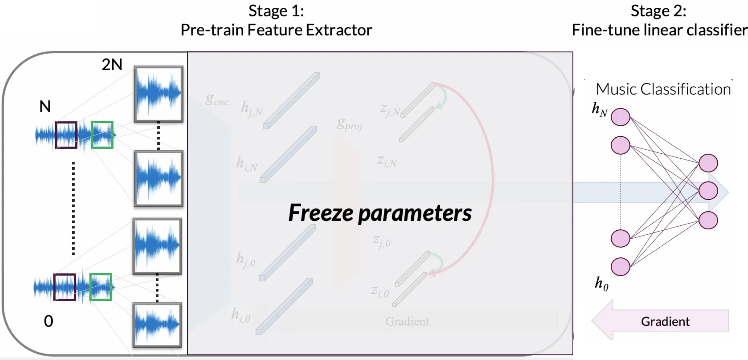
In the following examples, we will be taking a look at how Contrastive Learning of Musical Representations (Spijkervet & Burgoyne, 2021) uses self-supervised learning to learn powerful representations for the downstream task of music classification.
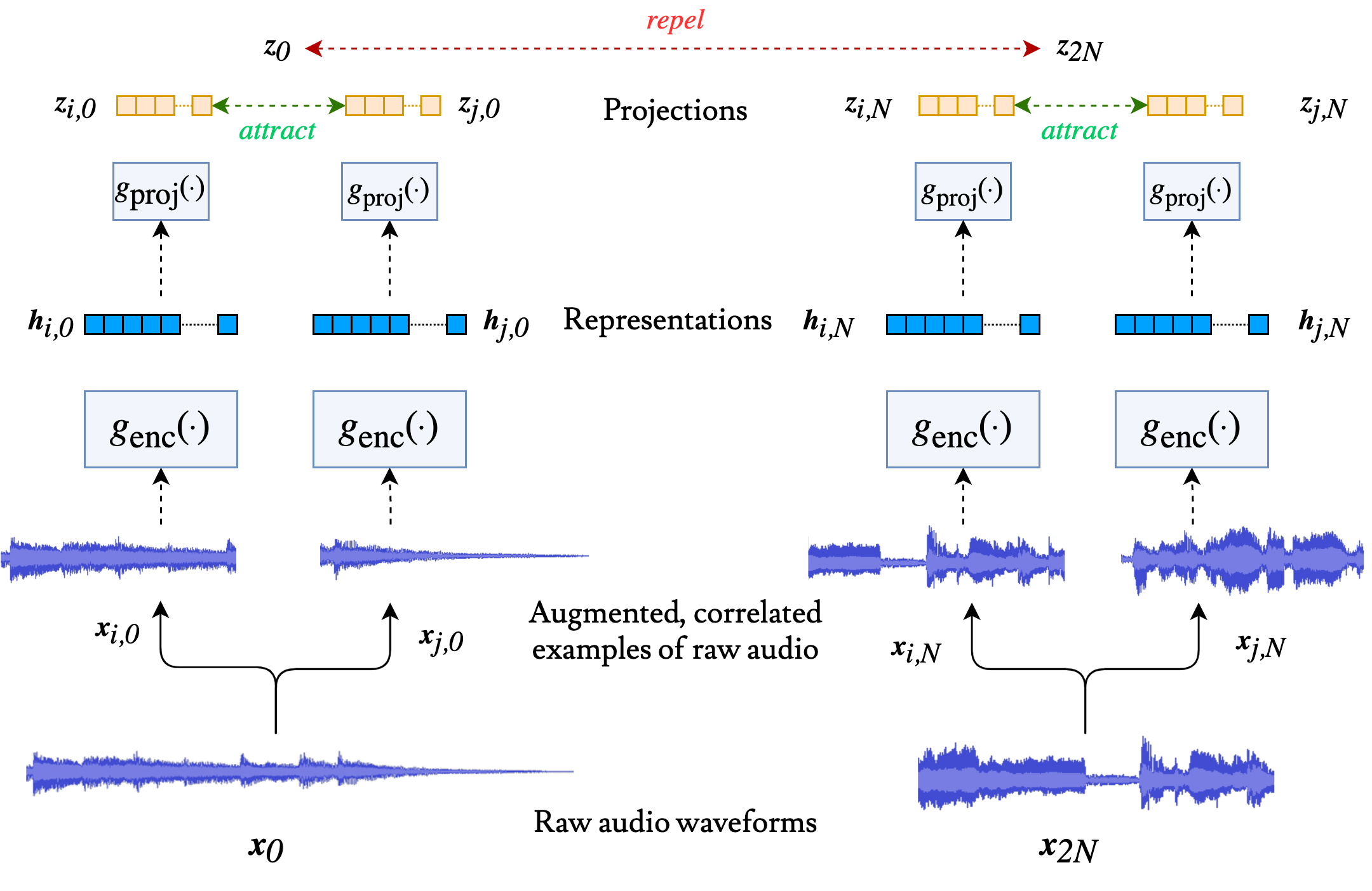
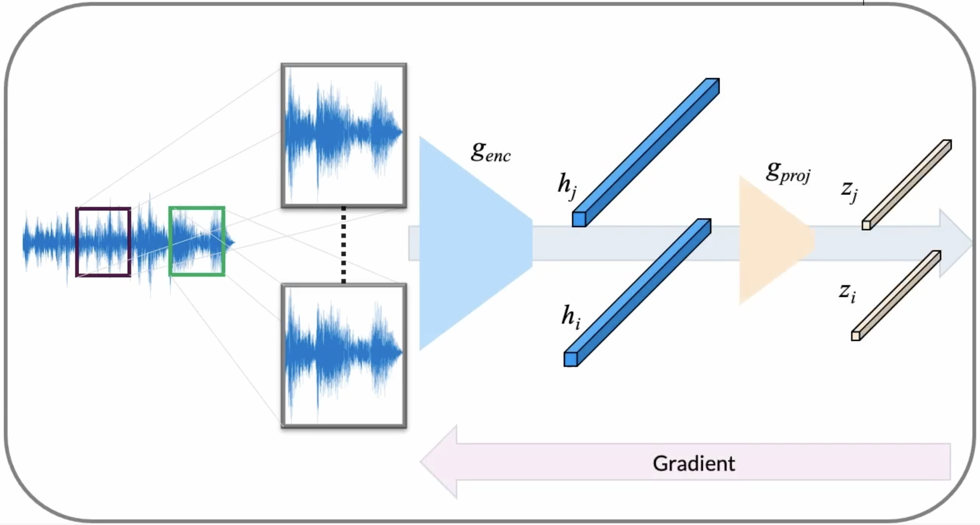
In the above figure, we transform a single audio example into two, distinct augmented views by processing it through a set of stochastic audio augmentations.
from argparse import Namespace

import torch
from tqdm import tqdm

device = torch.device("cuda") if torch.cuda.is_available() else torch.device("cpu")
print(f"We are using the following the device to train: {device}")

# initialize an empty argparse Namespace in which we can store argumens for training
args = Namespace()


# every piece of audio has a length of 59049 samples
args.audio_length = 59049

# the sample rate of our audio
args.sample_rate = 22050
We are using the following the device to train: cpu
import os
import random

import numpy as np
import soundfile as sf
import torch
from torch.utils import data
from torchaudio_augmentations import (
    Compose,
    Delay,
    Gain,
    HighLowPass,
    Noise,
    PitchShift,
    PolarityInversion,
    RandomApply,
    RandomResizedCrop,
    Reverb,
)

GTZAN_GENRES = [
    "blues",
    "classical",
    "country",
    "disco",
    "hiphop",
    "jazz",
    "metal",
    "pop",
    "reggae",
    "rock",
]


class GTZANDataset(data.Dataset):
    def __init__(self, data_path, split, num_samples, num_chunks, is_augmentation):
        self.data_path = data_path if data_path else ""
        self.split = split
        self.num_samples = num_samples
        self.num_chunks = num_chunks
        self.is_augmentation = is_augmentation
        self.genres = GTZAN_GENRES
        self._get_song_list()
        if is_augmentation:
            self._get_augmentations()

    def _get_song_list(self):
        list_filename = os.path.join(self.data_path, "%s_filtered.txt" % self.split)
        with open(list_filename) as f:
            lines = f.readlines()
        self.song_list = [line.strip() for line in lines]

    def _get_augmentations(self):
        transforms = [
            RandomResizedCrop(n_samples=self.num_samples),
            RandomApply([PolarityInversion()], p=0.8),
            RandomApply([Noise(min_snr=0.3, max_snr=0.5)], p=0.3),
            RandomApply([Gain()], p=0.2),
            RandomApply([HighLowPass(sample_rate=22050)], p=0.8),
            RandomApply([Delay(sample_rate=22050)], p=0.5),
            RandomApply(
                [PitchShift(n_samples=self.num_samples, sample_rate=22050)], p=0.4
            ),
            RandomApply([Reverb(sample_rate=22050)], p=0.3),
        ]
        self.augmentation = Compose(transforms=transforms)

    def _adjust_audio_length(self, wav):
        if self.split == "train":
            random_index = random.randint(0, len(wav) - self.num_samples - 1)
            wav = wav[random_index : random_index + self.num_samples]
        else:
            hop = (len(wav) - self.num_samples) // self.num_chunks
            wav = np.array(
                [
                    wav[i * hop : i * hop + self.num_samples]
                    for i in range(self.num_chunks)
                ]
            )
        return wav

    def get_augmentation(self, wav):
        return self.augmentation(torch.from_numpy(wav).unsqueeze(0)).squeeze(0).numpy()

    def __getitem__(self, index):
        line = self.song_list[index]

        # get genre
        genre_name = line.split("/")[0]
        genre_index = self.genres.index(genre_name)

        # get audio
        audio_filename = os.path.join(self.data_path, "genres", line)
        wav, fs = sf.read(audio_filename)

        # adjust audio length
        wav = self._adjust_audio_length(wav).astype("float32")

        # data augmentation
        if self.is_augmentation:
            wav_i = self.get_augmentation(wav)
            wav_j = self.get_augmentation(wav)
        else:
            wav_i = wav
            wav_j = wav

        return (wav_i, wav_j), genre_index

    def __len__(self):
        return len(self.song_list)


def get_dataloader(
    data_path=None,
    split="train",
    num_samples=22050 * 29,
    num_chunks=1,
    batch_size=16,
    num_workers=0,
    is_augmentation=False,
):
    is_shuffle = True if (split == "train") else False
    batch_size = batch_size if (split == "train") else (batch_size // num_chunks)
    data_loader = data.DataLoader(
        dataset=GTZANDataset(
            data_path, split, num_samples, num_chunks, is_augmentation
        ),
        batch_size=batch_size,
        shuffle=is_shuffle,
        drop_last=False,
        num_workers=num_workers,
    )
    return data_loader
args.batch_size = 48


train_loader = get_dataloader(
    data_path="../../codes/split",
    split="train",
    is_augmentation=True,
    num_samples=59049,
    batch_size=args.batch_size,
)
iter_train_loader = iter(train_loader)
(train_wav_i, _), train_genre = next(iter_train_loader)

valid_loader = get_dataloader(
    data_path="../../codes/split",
    split="valid",
    num_samples=args.audio_length,
    batch_size=args.batch_size,
)
test_loader = get_dataloader(
    data_path="../../codes/split",
    split="test",
    num_samples=args.audio_length,
    batch_size=args.batch_size,
)
iter_test_loader = iter(test_loader)
(test_wav_i, _), test_genre = next(iter_test_loader)
print("training data shape: %s" % str(train_wav_i.shape))
print("validation/test data shape: %s" % str(test_wav_i.shape))
print(train_genre)
Audio Data Augmentations
Now, let’s apply a series of transformations, each applied with an independent probability:
Crop
Filter
Reverb
Polarity
Noise
Pitch
Gain
Delay
import torchaudio
from torchaudio_augmentations import (
    RandomApply,
    ComposeMany,
    RandomResizedCrop,
    PolarityInversion,
    Noise,
    Gain,
    HighLowPass,
    Delay,
    PitchShift,
    Reverb,
)
args.transforms_polarity = 0.8
args.transforms_filters = 0.6
args.transforms_noise = 0.1
args.transforms_gain = 0.3
args.transforms_delay = 0.4
args.transforms_pitch = 0.4
args.transforms_reverb = 0.4


train_transform = [
    RandomResizedCrop(n_samples=args.audio_length),
    RandomApply([PolarityInversion()], p=args.transforms_polarity),
    RandomApply([Noise()], p=args.transforms_noise),
    RandomApply([Gain()], p=args.transforms_gain),
    RandomApply([HighLowPass(sample_rate=args.sample_rate)], p=args.transforms_filters),
    RandomApply([Delay(sample_rate=args.sample_rate)], p=args.transforms_delay),
    RandomApply([PitchShift(n_samples=args.audio_length, sample_rate=args.sample_rate)], p=args.transforms_pitch),
    RandomApply([Reverb(sample_rate=args.sample_rate)], p=args.transforms_reverb),
]
train_loader.augmentation = Compose(train_transform)
Remember, always take a moment to listen to the data that you will give to your model! Let’s listen to three examples from our dataset, on which a series of stochastic audio data augmentations are applied:
from IPython.display import Audio

for idx in range(3):
    print(f"Iteration: {idx}")
    (x_i, x_j), y = train_loader.dataset[0]

    print("Positive pair: (x_i, x_j):")
    display(Audio(x_i, rate=args.sample_rate))
    display(Audio(x_j, rate=args.sample_rate))
Iteration: 0
Positive pair: (x_i, x_j):
Iteration: 1
Positive pair: (x_i, x_j):
Iteration: 2
Positive pair: (x_i, x_j):
SampleCNN Encoder
First, let us begin with initializing our feature extractor. In CLMR, we chose the SampleCNN encoder to learn high-level features from raw pieces of audio. In the above figure, this encoder is denoted as $g_{enc}$. The last fully connected layer will be removed, so that we obtain an expressive final vector on which we can compute our contrastive loss.
import torch.nn as nn


class SampleCNN(nn.Module):
    def __init__(self, strides, supervised, out_dim):
        super(SampleCNN, self).__init__()

        self.strides = strides
        self.supervised = supervised
        self.sequential = [
            nn.Sequential(
                nn.Conv1d(1, 128, kernel_size=3, stride=3, padding=0),
                nn.BatchNorm1d(128),
                nn.ReLU(),
            )
        ]

        self.hidden = [
            [128, 128],
            [128, 128],
            [128, 256],
            [256, 256],
            [256, 256],
            [256, 256],
            [256, 256],
            [256, 256],
            [256, 512],
        ]

        assert len(self.hidden) == len(
            self.strides
        ), "Number of hidden layers and strides are not equal"
        for stride, (h_in, h_out) in zip(self.strides, self.hidden):
            self.sequential.append(
                nn.Sequential(
                    nn.Conv1d(h_in, h_out, kernel_size=stride, stride=1, padding=1),
                    nn.BatchNorm1d(h_out),
                    nn.ReLU(),
                    nn.MaxPool1d(stride, stride=stride),
                )
            )

        # 1 x 512
        self.sequential.append(
            nn.Sequential(
                nn.Conv1d(512, 512, kernel_size=3, stride=1, padding=1),
                nn.BatchNorm1d(512),
                nn.ReLU(),
            )
        )

        self.sequential = nn.Sequential(*self.sequential)

        if self.supervised:
            self.dropout = nn.Dropout(0.5)
        self.fc = nn.Linear(512, out_dim)

    def initialize(self, m):
        if isinstance(m, (nn.Conv1d)):
            nn.init.kaiming_uniform_(m.weight, mode="fan_in", nonlinearity="relu")

    def forward(self, x):
        x = x.unsqueeze(dim=1)  # here, we add a dimension for our convolution.
        out = self.sequential(x)
        if self.supervised:
            out = self.dropout(out)

        out = out.reshape(x.shape[0], out.size(1) * out.size(2))
        logit = self.fc(out)
        return logit
Let’s have a look at a printed version of SampleCNN:
# in the GTZAN dataset, we have 10 genre labels
args.n_classes = 10

encoder = SampleCNN(
    strides=[3, 3, 3, 3, 3, 3, 3, 3, 3],
    supervised=False,
    out_dim=args.n_classes,
).to(device)
print(encoder)
SampleCNN(
  (sequential): Sequential(
    (0): Sequential(
      (0): Conv1d(1, 128, kernel_size=(3,), stride=(3,))
      (1): BatchNorm1d(128, eps=1e-05, momentum=0.1, affine=True, track_running_stats=True)
      (2): ReLU()
    )
    (1): Sequential(
      (0): Conv1d(128, 128, kernel_size=(3,), stride=(1,), padding=(1,))
      (1): BatchNorm1d(128, eps=1e-05, momentum=0.1, affine=True, track_running_stats=True)
      (2): ReLU()
      (3): MaxPool1d(kernel_size=3, stride=3, padding=0, dilation=1, ceil_mode=False)
    )
    (2): Sequential(
      (0): Conv1d(128, 128, kernel_size=(3,), stride=(1,), padding=(1,))
      (1): BatchNorm1d(128, eps=1e-05, momentum=0.1, affine=True, track_running_stats=True)
      (2): ReLU()
      (3): MaxPool1d(kernel_size=3, stride=3, padding=0, dilation=1, ceil_mode=False)
    )
    (3): Sequential(
      (0): Conv1d(128, 256, kernel_size=(3,), stride=(1,), padding=(1,))
      (1): BatchNorm1d(256, eps=1e-05, momentum=0.1, affine=True, track_running_stats=True)
      (2): ReLU()
      (3): MaxPool1d(kernel_size=3, stride=3, padding=0, dilation=1, ceil_mode=False)
    )
    (4): Sequential(
      (0): Conv1d(256, 256, kernel_size=(3,), stride=(1,), padding=(1,))
      (1): BatchNorm1d(256, eps=1e-05, momentum=0.1, affine=True, track_running_stats=True)
      (2): ReLU()
      (3): MaxPool1d(kernel_size=3, stride=3, padding=0, dilation=1, ceil_mode=False)
    )
    (5): Sequential(
      (0): Conv1d(256, 256, kernel_size=(3,), stride=(1,), padding=(1,))
      (1): BatchNorm1d(256, eps=1e-05, momentum=0.1, affine=True, track_running_stats=True)
      (2): ReLU()
      (3): MaxPool1d(kernel_size=3, stride=3, padding=0, dilation=1, ceil_mode=False)
    )
    (6): Sequential(
      (0): Conv1d(256, 256, kernel_size=(3,), stride=(1,), padding=(1,))
      (1): BatchNorm1d(256, eps=1e-05, momentum=0.1, affine=True, track_running_stats=True)
      (2): ReLU()
      (3): MaxPool1d(kernel_size=3, stride=3, padding=0, dilation=1, ceil_mode=False)
    )
    (7): Sequential(
      (0): Conv1d(256, 256, kernel_size=(3,), stride=(1,), padding=(1,))
      (1): BatchNorm1d(256, eps=1e-05, momentum=0.1, affine=True, track_running_stats=True)
      (2): ReLU()
      (3): MaxPool1d(kernel_size=3, stride=3, padding=0, dilation=1, ceil_mode=False)
    )
    (8): Sequential(
      (0): Conv1d(256, 256, kernel_size=(3,), stride=(1,), padding=(1,))
      (1): BatchNorm1d(256, eps=1e-05, momentum=0.1, affine=True, track_running_stats=True)
      (2): ReLU()
      (3): MaxPool1d(kernel_size=3, stride=3, padding=0, dilation=1, ceil_mode=False)
    )
    (9): Sequential(
      (0): Conv1d(256, 512, kernel_size=(3,), stride=(1,), padding=(1,))
      (1): BatchNorm1d(512, eps=1e-05, momentum=0.1, affine=True, track_running_stats=True)
      (2): ReLU()
      (3): MaxPool1d(kernel_size=3, stride=3, padding=0, dilation=1, ceil_mode=False)
    )
    (10): Sequential(
      (0): Conv1d(512, 512, kernel_size=(3,), stride=(1,), padding=(1,))
      (1): BatchNorm1d(512, eps=1e-05, momentum=0.1, affine=True, track_running_stats=True)
      (2): ReLU()
    )
  )
  (fc): Linear(in_features=512, out_features=10, bias=True)
)
SimCLR
Since we removed the last fully connected layer, we are left with a $512$-dimensional feature vector. We would like to use this vector in our contrastive learning task. Therefore, we wrap our encoder in the objective as introduced by SimCLR: we project the final hidden layer of the encoder to a different latent space using a small MLP projector network. In the forward pass, we extract both the final hidden representation of our SampleCNN encoder (h_i and h_j), and the projected vectors (z_i and z_j).
class SimCLR(nn.Module):
    def __init__(self, encoder, projection_dim, n_features):
        super(SimCLR, self).__init__()

        self.encoder = encoder
        self.n_features = n_features

        # Replace the fc layer with an Identity function
        self.encoder.fc = Identity()

        # We use a MLP with one hidden layer to obtain z_i = g(h_i) = W(2)σ(W(1)h_i) where σ is a ReLU non-linearity.
        self.projector = nn.Sequential(
            nn.Linear(self.n_features, self.n_features, bias=False),
            nn.ReLU(),
            nn.Linear(self.n_features, projection_dim, bias=False),
        )

    def forward(self, x_i, x_j):
        h_i = self.encoder(x_i)
        h_j = self.encoder(x_j)

        z_i = self.projector(h_i)
        z_j = self.projector(h_j)
        return h_i, h_j, z_i, z_j


class Identity(nn.Module):
    def __init__(self):
        super(Identity, self).__init__()

    def forward(self, x):
        return x
Loss
Here, we apply an InfoNCE loss, as proposed by van den Oord et al. (2018) for contrastive learning. InfoNCE loss compares the similarity of our representations $z_i$ and $z_j$, to the similarity of $z_i$ to any other representation in our batch, and applies a softmax over the obtained similarity values. We can write this loss more formally as follows:

The similarity metric is the cosine similarity between our representations:

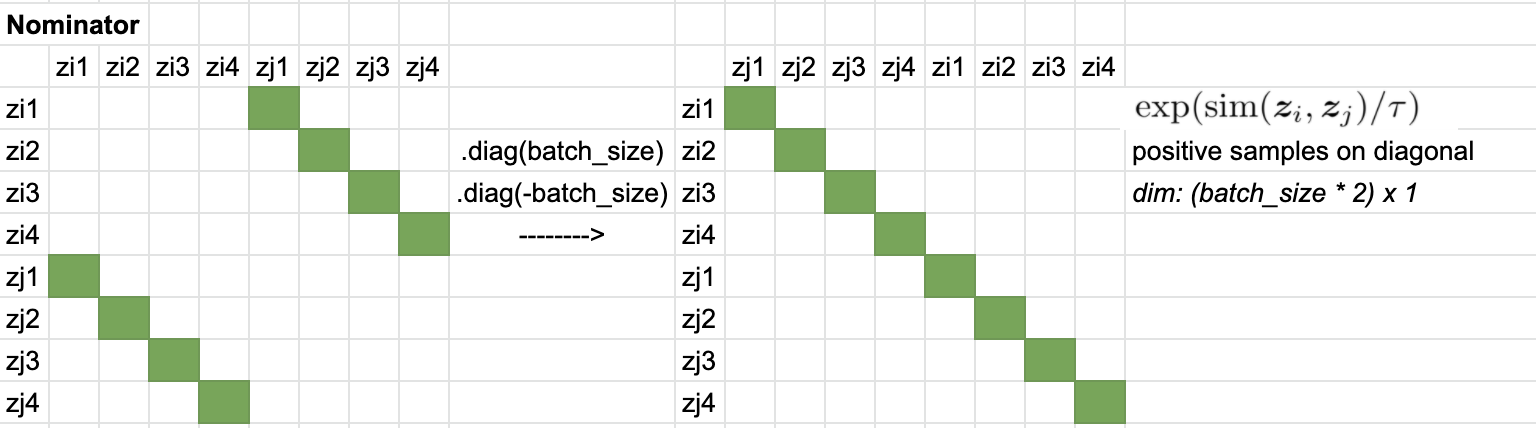
z = torch.cat((z_i, z_j), dim=0)`
sim = self.similarity_f(z.unsqueeze(1), z.unsqueeze(0)) / self.temperature
sim_i_j = torch.diag(sim, self.batch_size * self.world_size)
sim_j_i = torch.diag(sim, -self.batch_size * self.world_size)
positive_samples = torch.cat((sim_i_j, sim_j_i), dim=0).reshape(N, 1)
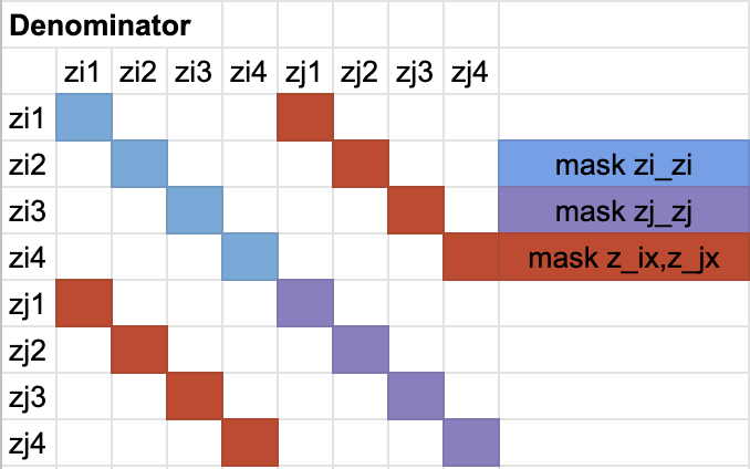
negative_samples = sim[self.mask].reshape(N, -1)
import torch
import torch.nn as nn


class NT_Xent(nn.Module):
    def __init__(self, batch_size, temperature, world_size):
        super(NT_Xent, self).__init__()
        self.batch_size = batch_size
        self.temperature = temperature
        self.world_size = world_size

        self.mask = self.mask_correlated_samples(batch_size, world_size)
        self.criterion = nn.CrossEntropyLoss(reduction="sum")
        self.similarity_f = nn.CosineSimilarity(dim=2)

    def mask_correlated_samples(self, batch_size, world_size):
        N = 2 * batch_size * world_size
        mask = torch.ones((N, N), dtype=bool)
        mask = mask.fill_diagonal_(0)
        for i in range(batch_size * world_size):
            mask[i, batch_size * world_size + i] = 0
            mask[batch_size * world_size + i, i] = 0
        return mask

    def forward(self, z_i, z_j):
        """
        We do not sample negative examples explicitly.
        Instead, given a positive pair, similar to (Chen et al., 2017), we treat the other 2(N − 1) augmented examples within a minibatch as negative examples.
        """
        N = 2 * self.batch_size * self.world_size

        z = torch.cat((z_i, z_j), dim=0)

        sim = self.similarity_f(z.unsqueeze(1), z.unsqueeze(0)) / self.temperature

        sim_i_j = torch.diag(sim, self.batch_size * self.world_size)
        sim_j_i = torch.diag(sim, -self.batch_size * self.world_size)

        # We have 2N samples, but with Distributed training every GPU gets N examples too, resulting in: 2xNxN
        positive_samples = torch.cat((sim_i_j, sim_j_i), dim=0).reshape(N, 1)
        negative_samples = sim[self.mask].reshape(N, -1)

        labels = torch.zeros(N).to(positive_samples.device).long()
        logits = torch.cat((positive_samples, negative_samples), dim=1)
        loss = self.criterion(logits, labels)
        loss /= N
        return loss
Pre-training CLMR

Note
The following code will pre-train our SampleCNN encoder using our contrastive loss. This needs to run on a machine with a GPU to accelerate training, otherwise it will take a very long time.
args.temperature = 0.5  # the temperature scaling parameter in our NT-Xent los


encoder = SampleCNN(
    strides=[3, 3, 3, 3, 3, 3, 3, 3, 3],
    supervised=False,
    out_dim=0,
).to(device)


# get dimensions of last fully-connected layer
n_features = encoder.fc.in_features
print(f"Dimension of our h_i, h_j vectors: {n_features}")

model = SimCLR(encoder, projection_dim=64, n_features=n_features).to(device)

temperature = 0.5
optimizer = torch.optim.Adam(model.parameters(), lr=3e-4)
criterion = NT_Xent(args.batch_size, args.temperature, world_size=1)

epochs = 100
losses = []

for e in range(epochs):

    for (x_i, x_j), y in train_loader:
        optimizer.zero_grad()

        x_i = x_i.to(device)
        x_j = x_j.to(device)

        # here, we extract the latent representations, and the projected vectors,
        # from the positive pairs:
        h_i, h_j, z_i, z_j = model(x_i, x_j)

        # here, we calculate the NT-Xent loss on the projected vectors:
        loss = criterion(z_i, z_j)

        # backpropagation:
        loss.backward()
        optimizer.step()

        print(f"Loss: {loss}")
        losses.append(loss.detach().item())

        break  # we are only running a single pass for demonstration purposes.

    print(f"Mean loss: {np.array(losses).mean()}")
    break  # we are only running a single epoch for demonstration purposes.
Dimension of our h_i, h_j vectors: 512
Loss: 2.5802388191223145
Mean loss: 2.5802388191223145
Linear Evaluation
Now, we would like to evaluate the versatility of our learned representations. We will train a linear classifier on the representations extracted from our pre-trained SampleCNN encoder.
Warning
Note that we will not be using data augmentations during linear evaluation.
args.batch_size = 16


train_loader = get_dataloader(
    data_path="../../codes/split",
    split="train",
    is_augmentation=False,
    num_samples=args.audio_length,
    batch_size=args.batch_size,
)
valid_loader = get_dataloader(
    data_path="../../codes/split",
    split="valid",
    num_samples=args.audio_length,
    batch_size=args.batch_size,
)
test_loader = get_dataloader(
    data_path="../../codes/split",
    split="test",
    num_samples=args.audio_length,
    batch_size=args.batch_size,
)

iter_train_loader = iter(train_loader)
iter_test_loader = iter(test_loader)


for idx in range(3):
    (train_wav, _), train_genre = train_loader.dataset[idx]
    display(Audio(train_wav, rate=args.sample_rate))
Our linear classifier has a single hidden layer and a softmax output (which is already included in the torch.nn.CrossEntropy loss function, hence we omit it here).
class LinearModel(nn.Module):
    def __init__(self, hidden_dim, output_dim):
        super().__init__()
        self.hidden_dim = hidden_dim
        self.output_dim = output_dim
        self.model = nn.Linear(self.hidden_dim, self.output_dim)

    def forward(self, x):
        return self.model(x)
def train_linear_model(encoder, linear_model, epochs, learning_rate):

    # we now use a regular CrossEntropy loss to compare our predicted genre labels with the ground truth labels.
    criterion = nn.CrossEntropyLoss()

    # the Adam optimizer is used here as our optimization algorithm
    optimizer = torch.optim.Adam(
        linear_model.parameters(),
        lr=learning_rate,
    )

    losses = []
    for e in range(epochs):
        epoch_losses = []
        for (x, _), y in tqdm(train_loader):

            optimizer.zero_grad()

            # we will not be backpropagating the gradients of the SampleCNN encoder:
            with torch.no_grad():
                h = encoder(x)

            p = linear_model(h)

            loss = criterion(p, y)

            loss.backward()
            optimizer.step()

            # print(f"Loss: {loss}")
            epoch_losses.append(loss.detach().item())

        mean_loss = np.array(epoch_losses).mean()
        losses.append(mean_loss)
        print(f"Epoch: {e}\tMean loss: {mean_loss}")
    return losses
args.linear_learning_rate = 1e-4
args.linear_epochs = 15
print(f"We will train for {args.linear_epochs} epochs during linear evaluation")


# First, we freeze SampleCNN encoder weights
encoder.eval()
for param in encoder.parameters():
    param.requires_grad = False

print(
    f"Dimension of the last layer of our SampleCNN feature extractor network: {n_features}"
)


# initialize our linear model, with dimensions:
# n_features x n_classes

linear_model = LinearModel(n_features, args.n_classes)
print(linear_model)

losses = train_linear_model(
    encoder,
    linear_model,
    epochs=args.linear_epochs,
    learning_rate=args.linear_learning_rate,
)
We will train for 15 epochs during linear evaluation
Dimension of the last layer of our SampleCNN feature extractor network: 512
LinearModel(
  (model): Linear(in_features=512, out_features=10, bias=True)
)
100%|███████████████████████████████████████████████████████████████████████████████████████████████████| 28/28 [00:37<00:00, 1.33s/it]
Epoch: 0 Mean loss: 2.3029658624104092
100%|███████████████████████████████████████████████████████████████████████████████████████████████████| 28/28 [00:37<00:00, 1.33s/it]
Epoch: 1 Mean loss: 2.3026398164885387
100%|███████████████████████████████████████████████████████████████████████████████████████████████████| 28/28 [00:37<00:00, 1.34s/it]
Epoch: 2 Mean loss: 2.302783123084477
100%|███████████████████████████████████████████████████████████████████████████████████████████████████| 28/28 [00:37<00:00, 1.34s/it]
Epoch: 3 Mean loss: 2.302727324622018
100%|███████████████████████████████████████████████████████████████████████████████████████████████████| 28/28 [00:37<00:00, 1.34s/it]
Epoch: 4 Mean loss: 2.302577691418784
100%|███████████████████████████████████████████████████████████████████████████████████████████████████| 28/28 [00:37<00:00, 1.34s/it]
Epoch: 5 Mean loss: 2.3024674568857466
100%|███████████████████████████████████████████████████████████████████████████████████████████████████| 28/28 [00:37<00:00, 1.34s/it]
Epoch: 6 Mean loss: 2.3024762954030717
100%|███████████████████████████████████████████████████████████████████████████████████████████████████| 28/28 [00:37<00:00, 1.35s/it]
Epoch: 7 Mean loss: 2.302462100982666
100%|███████████████████████████████████████████████████████████████████████████████████████████████████| 28/28 [00:38<00:00, 1.36s/it]
Epoch: 8 Mean loss: 2.302406898566655
100%|███████████████████████████████████████████████████████████████████████████████████████████████████| 28/28 [00:38<00:00, 1.36s/it]
Epoch: 9 Mean loss: 2.3019944769995555
100%|███████████████████████████████████████████████████████████████████████████████████████████████████| 28/28 [00:38<00:00, 1.36s/it]
Epoch: 10 Mean loss: 2.302449566977365
100%|███████████████████████████████████████████████████████████████████████████████████████████████████| 28/28 [00:38<00:00, 1.36s/it]
Epoch: 11 Mean loss: 2.3020790219306946
100%|███████████████████████████████████████████████████████████████████████████████████████████████████| 28/28 [00:38<00:00, 1.36s/it]
Epoch: 12 Mean loss: 2.301789471081325
100%|███████████████████████████████████████████████████████████████████████████████████████████████████| 28/28 [00:38<00:00, 1.36s/it]
Epoch: 13 Mean loss: 2.302112783704485
100%|███████████████████████████████████████████████████████████████████████████████████████████████████| 28/28 [00:38<00:00, 1.36s/it]
Epoch: 14 Mean loss: 2.3021752067974637
In the evaluate function, we perform a full pass of the test dataset and extract the predictions from our linear classifier, given the representations of our pre-trained encoder.
# Run evaluation


def evaluate(encoder, linear_model=None, test_loader=None):
    encoder.eval()
    if linear_model is not None:
        linear_model.eval()

    y_true = []
    y_pred = []

    with torch.no_grad():
        for (wav, _), genre_index in tqdm(test_loader):
            wav = wav.to(device)
            genre_index = genre_index.to(device)

            # reshape and aggregate chunk-level predictions
            b, c, t = wav.size()

            with torch.no_grad():
                if linear_model is None:
                    logits = encoder(wav.squeeze(1))
                else:
                    h = encoder(wav.squeeze(1))
                    logits = linear_model(h)

            logits = logits.view(b, c, -1).mean(dim=1)
            _, pred = torch.max(logits.data, 1)

            # append labels and predictions
            y_true.extend(genre_index.tolist())
            y_pred.extend(pred.tolist())

    return y_true, y_pred
import seaborn as sns
from sklearn.metrics import accuracy_score, confusion_matrix
y_true, y_pred = evaluate(encoder, linear_model, test_loader)
accuracy = accuracy_score(y_true, y_pred)
cm = confusion_matrix(y_true, y_pred)
sns.heatmap(
cm, annot=True, xticklabels=GTZAN_GENRES, yticklabels=GTZAN_GENRES, cmap="YlGnBu"
)
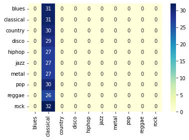
print("Accuracy: %.4f" % accuracy)
100%|███████████████████████████████████████████████████████████████████████████████████████████████████| 19/19 [00:26<00:00, 1.39s/it]
Accuracy: 0.1069
We can also load the weights of a fully pre-trained CLMR model to our SampleCNN encoder. The pre-trained representations will hopefully be more expressive for the linear classifier to solve the problem of music classification.
Note
Pre-training the encoder takes a while to complete, so let’s load the pre-trained weights into our encoder now to speed this up:
from collections import OrderedDict

pre_trained_weights = torch.load("./clmr_pretrained.ckpt", map_location=device)

# this dictionary contains a few parameters we do not need  in this tutorial, so we discard them here:
pre_trained_weights = OrderedDict(
    {
        k.replace("encoder.", ""): v
        for k, v in pre_trained_weights.items()
        if "encoder" in k
    }
)


# let's load the weights into our encoder:
encoder = SampleCNN(
    strides=[3, 3, 3, 3, 3, 3, 3, 3, 3],
    supervised=False,
    out_dim=0,
).to(device)
encoder.fc = Identity()
encoder.load_state_dict(pre_trained_weights)
encoder.eval()

# we re-initialize our linear model here to discard the previously learned parameters.
linear_model = LinearModel(n_features, args.n_classes)
losses_with_clmr = train_linear_model(
    encoder,
    linear_model,
    epochs=args.linear_epochs,
    learning_rate=args.linear_learning_rate,
)
/Users/janne/miniconda3/envs/tutorial/lib/python3.8/site-packages/torch/nn/init.py:388: UserWarning: Initializing zero-element tensors is a no-op
  warnings.warn("Initializing zero-element tensors is a no-op")
100%|███████████████████████████████████████████████████████████████████████████████████████████████████| 28/28 [00:38<00:00,  1.38s/it]
Epoch: 0 Mean loss: 2.340274861880711
100%|███████████████████████████████████████████████████████████████████████████████████████████████████| 28/28 [00:38<00:00, 1.36s/it]
Epoch: 1 Mean loss: 2.1566108635493686
100%|███████████████████████████████████████████████████████████████████████████████████████████████████| 28/28 [00:38<00:00, 1.36s/it]
Epoch: 2 Mean loss: 2.0396491161414554
100%|███████████████████████████████████████████████████████████████████████████████████████████████████| 28/28 [00:38<00:00, 1.37s/it]
Epoch: 3 Mean loss: 1.948716210467475
100%|███████████████████████████████████████████████████████████████████████████████████████████████████| 28/28 [00:38<00:00, 1.36s/it]
Epoch: 4 Mean loss: 1.871069073677063
100%|███████████████████████████████████████████████████████████████████████████████████████████████████| 28/28 [00:38<00:00, 1.37s/it]
Epoch: 5 Mean loss: 1.7560220999377114
100%|███████████████████████████████████████████████████████████████████████████████████████████████████| 28/28 [00:38<00:00, 1.37s/it]
Epoch: 6 Mean loss: 1.6884811690875463
100%|███████████████████████████████████████████████████████████████████████████████████████████████████| 28/28 [00:38<00:00, 1.36s/it]
Epoch: 7 Mean loss: 1.6221486585480827
100%|███████████████████████████████████████████████████████████████████████████████████████████████████| 28/28 [00:38<00:00, 1.36s/it]
Epoch: 8 Mean loss: 1.5455367820603507
100%|███████████████████████████████████████████████████████████████████████████████████████████████████| 28/28 [00:38<00:00, 1.37s/it]
Epoch: 9 Mean loss: 1.4933379547936576
100%|███████████████████████████████████████████████████████████████████████████████████████████████████| 28/28 [00:38<00:00, 1.36s/it]
Epoch: 10 Mean loss: 1.4579386711120605
100%|███████████████████████████████████████████████████████████████████████████████████████████████████| 28/28 [00:38<00:00, 1.37s/it]
Epoch: 11 Mean loss: 1.3922432788780756
100%|███████████████████████████████████████████████████████████████████████████████████████████████████| 28/28 [00:38<00:00, 1.37s/it]
Epoch: 12 Mean loss: 1.3564506087984358
100%|███████████████████████████████████████████████████████████████████████████████████████████████████| 28/28 [00:38<00:00, 1.37s/it]
Epoch: 13 Mean loss: 1.3168576232024602
100%|███████████████████████████████████████████████████████████████████████████████████████████████████| 28/28 [00:38<00:00, 1.37s/it]
Epoch: 14 Mean loss: 1.270722210407257
Get ROC-AUC and PR-AUC scores on test set
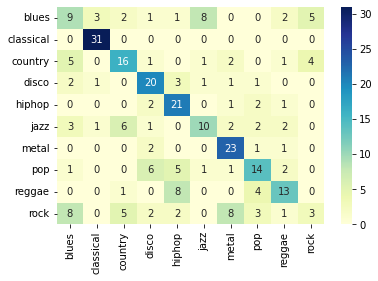
Let’s now compute the accuracy of a linear classifier, trained on the representations from a pre-trained CLMR model.
y_true_pretrained, y_pred_pretrained = evaluate(encoder, linear_model, test_loader)

pretrained_accuracy = accuracy_score(y_true_pretrained, y_pred_pretrained)
cm = confusion_matrix(y_true_pretrained, y_pred_pretrained)
sns.heatmap(
    cm, annot=True, xticklabels=GTZAN_GENRES, yticklabels=GTZAN_GENRES, cmap="YlGnBu"
)
print("Accuracy: %.4f" % pretrained_accuracy)
100%|███████████████████████████████████████████████████████████████████████████████████████████████████| 19/19 [00:25<00:00, 1.33s/it]
Accuracy: 0.5517
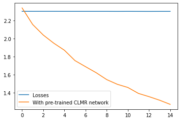
import matplotlib.pyplot as plt

plt.plot(losses, label="Losses")
plt.plot(losses_with_clmr, label="With pre-trained CLMR network")
plt.legend()
plt.show()
How does a supervised SampleCNN model compare?
# let's load the weights into our encoder:
supervised_samplecnn = SampleCNN(
    strides=[3, 3, 3, 3, 3, 3, 3, 3, 3],
    supervised=True,
    out_dim=args.n_classes,
).to(device)

optimizer = torch.optim.Adam(supervised_samplecnn.parameters(), lr=3e-4)
criterion = nn.CrossEntropyLoss()

epochs = 15
losses = []
for e in range(epochs):
    epoch_losses = []
    for (x, _), y in tqdm(train_loader):
        optimizer.zero_grad()
        logits = supervised_samplecnn(x)

        # here, we calculate the NT-Xent loss on the projected vectors:
        loss = criterion(logits, y)

        # backpropagation:
        loss.backward()
        optimizer.step()

        # print(f"Loss: {loss}")
        epoch_losses.append(loss.detach().item())

    mean_loss = np.array(epoch_losses).mean()
    losses.append(mean_loss)
    print(f"Epoch: {e}\tMean loss: {mean_loss}")
100%|███████████████████████████████████████████████████████████████████████████████████████████████████| 28/28 [01:59<00:00, 4.25s/it]
Epoch: 0 Mean loss: 2.0514306170599803
100%|███████████████████████████████████████████████████████████████████████████████████████████████████| 28/28 [01:59<00:00, 4.26s/it]
Epoch: 1 Mean loss: 1.777217332805906
100%|███████████████████████████████████████████████████████████████████████████████████████████████████| 28/28 [02:00<00:00, 4.29s/it]
Epoch: 2 Mean loss: 1.6308889814785548
100%|███████████████████████████████████████████████████████████████████████████████████████████████████| 28/28 [02:00<00:00, 4.29s/it]
Epoch: 3 Mean loss: 1.508283602339881
100%|███████████████████████████████████████████████████████████████████████████████████████████████████| 28/28 [02:02<00:00, 4.38s/it]
Epoch: 4 Mean loss: 1.4906416535377502
100%|███████████████████████████████████████████████████████████████████████████████████████████████████| 28/28 [01:57<00:00, 4.20s/it]
Epoch: 5 Mean loss: 1.4243347091334206
100%|███████████████████████████████████████████████████████████████████████████████████████████████████| 28/28 [02:00<00:00, 4.31s/it]
Epoch: 6 Mean loss: 1.3204487540892191
100%|███████████████████████████████████████████████████████████████████████████████████████████████████| 28/28 [01:56<00:00, 4.16s/it]
Epoch: 7 Mean loss: 1.2581013866833277
100%|███████████████████████████████████████████████████████████████████████████████████████████████████| 28/28 [01:56<00:00, 4.15s/it]
Epoch: 8 Mean loss: 1.3584619547639574
100%|███████████████████████████████████████████████████████████████████████████████████████████████████| 28/28 [01:56<00:00, 4.16s/it]
Epoch: 9 Mean loss: 1.2448890315634864
100%|███████████████████████████████████████████████████████████████████████████████████████████████████| 28/28 [01:56<00:00, 4.16s/it]
Epoch: 10 Mean loss: 1.2725025245121546
100%|███████████████████████████████████████████████████████████████████████████████████████████████████| 28/28 [01:57<00:00, 4.18s/it]
Epoch: 11 Mean loss: 1.2021435052156448
100%|███████████████████████████████████████████████████████████████████████████████████████████████████| 28/28 [01:57<00:00, 4.19s/it]
Epoch: 12 Mean loss: 1.159744279725211
100%|███████████████████████████████████████████████████████████████████████████████████████████████████| 28/28 [01:57<00:00, 4.19s/it]
Epoch: 13 Mean loss: 1.1804143616131373
100%|███████████████████████████████████████████████████████████████████████████████████████████████████| 28/28 [01:58<00:00, 4.24s/it]
Epoch: 14 Mean loss: 1.0627801907914025
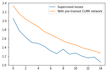
plt.plot(losses, label="Supervised losses")
plt.plot(losses_with_clmr, label="With pre-trained CLMR network")
plt.legend()
plt.show()
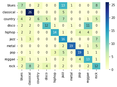
y_true_supervised, y_pred_supervised = evaluate(
    supervised_samplecnn, linear_model=None, test_loader=test_loader
)

supervised_accuracy = accuracy_score(y_true_supervised, y_pred_supervised)
cm = confusion_matrix(y_true_supervised, y_pred_supervised)
sns.heatmap(
    cm, annot=True, xticklabels=GTZAN_GENRES, yticklabels=GTZAN_GENRES, cmap="YlGnBu"
)
print("Accuracy: %.4f" % supervised_accuracy)
100%|███████████████████████████████████████████████████████████████████████████████████████████████████| 19/19 [00:26<00:00, 1.41s/it]
Accuracy: 0.4966
Conclusion
In conclusion, we observed how a self-supervised model, that pre-trains its network by way of leveraging the underlying structure of the data, can learn strong representations for the downstream task of music classification.
We have:
Pre-trained a SampleCNN encoder with CLMR.
Evaluated the representations with a linear classifier.
Loaded pre-trained weights from CLMR trained on the MagnaTagATune dataset.
Trained a linear classifier on these representations.
Our final accuracy when training the linear classifier for 15 epochs is ~55.2% on the downstream task of music classification on the GTZAN dataset.
It is important compare against an equivalent network that is trained in a supervised manner. Therefore, we also trained a supervised SampleCNN model from scratch, which reached an accuracy of ~49.6%.
Model |
Accuracy |
|---|---|
Supervised SampleCNN |
49.6% |
Self-supervised CLMR + SampleCNN |
55.2% |
Note
Note that in these experiments, the supervised model may have well overfitted on the GTZAN training data. This tutorial is by no means an exhaustive search for an optimal set of model and training parameters.
In conclusion, it is exciting to see that a linear classifier reaches a comparable performance, compared to a fully optimized encoder, using representations that were learned in a task-agnostic manner by way of self-supervised learning.